Energy Modeling
Historically the only purpose for modeling was to size heating and cooling systems, but now its used to tradeoff insulation amount, window efficiency and air tightness with HVAC/solar array sizes. Modeling also allows you to compare to a standard such as LEED, PassiveHouse, or standard construction via a HERS rating, if you happen to be interested in such comparisons, as well as determine how much PV you'll need if you want to be a zero-energy house. Modeling will also tell you how much passive solar gain you'll get, as well as whether you're getting too much in the summer. You can also get an estimate of what your yearly energy consumption will be.
Modeling energy use is theoretically simple, but practically complex, particularly over longer time periods. Occupant behavior such as thermostat setting, opening windows, and equipment use have a very large effect on building energy use. Likewise, energy use literally changes with the weather. On top of all this, add in radiant heat/loss gain (see discussions in the R-values section and heatflow section), and that fact that real-world assembly R-values vary somewhat from theoretical ones (see next section).
There are numerous software packages that calculate heat loss (including some free ones), some of which can do some very sophisticated modeling in an attempt to deal with the practical complications. Different programs have different capabilities, so the best one depends on what you want out of it. Even if you do buy a package, keep in mind that annual energy use is so dependent on occupant behavior and weather, no model can possibly predict the end result accurately.1 The more sophisticated packages will take more effects into account and hence get a better estimate, but you can still get useful estimates with just a simple model done in a spreadsheet.
If the concern is only ballpark yearly energy use, or only worst case energy use (for example to size a backup heating system), or typical case energy use, a simple spreadsheet will give a good result. The rest of the document describes how to do this, and explains the limitations of this approach.
Heat Loss = Conduction + infiltration
There are two primary methods of heat loss in building, conduction thru the building envelope (ie the exterior surface: floor, walls, roof, windows, etc) and via air infiltration (or rather warm air escaping the building being replaced by cold outside air). Other factors, such as radiant loss/gain really only affect the temperature difference from inside to out. Those factors can be quite significant for short periods of time, and may even significantly affect the yearly amount, but are ignored here.2
Heat loss thru the envelope
The general heat loss formula is: Q=U*A*ΔT, or in plain words, the heat loss of an area of size A is determined by the U value of the materials and the difference in temperature between inside and out (that is the difference in temperature of the two surfaces, not the two air temperatures, which might not be quite the same. Below is an adjustment for air temperatures.)
To get the heat loss of an entire building, you divide the building into areas that have the same U value, and then add them all up to get the total heat loss. So typically you will end up with four different areas: walls, windows & doors, roof and floor. If one of those areas had parts that have a different U value (for example a wall bump out that is constructed differently), you will end up breaking that into its own category also.
Heat loss thru an
assembly:
Because walls, roofs etc are assemblies of different materials, calculating
heat loss thru that assembly requires combining the R-values of the various
materials to calculate an effective R-value for the assembly.
First, divide the assembly into sections that are uniform from inside to outside, for example in a 2x4 wall, there is the part where insulation fills the cavity and the part where there is a 2x4 and no insulation.
Second, calculate the R-value of each section by adding of the R-values of each of its layers. For example, a typical 2x4 wall would be: R.5(wood siding)+R.5( 1/2" wood sheathing)+R11(insulation)+R.5(sheetrock)=R12.5. The R value of a material is either found in a table for the entire material(eg an R11 fiberglass batt which is 3.5" thick), or by using the R value per inch of material (eg R3.1/inch) and multiplying by the actual thickness (R3.1/inch*3.5inches=R11).
Third, calculate the U value of the assembly as the sum of the weighted U values of each section. To do this, you will first need to calculate what percentage of the total area each of the different sections occupy.
Uassembly = U1*%area1 + U2*%area2+...
The R value of the assembly is then just the inverse of its U-value.
Here is an example:
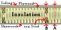 The
example wall section at right consists of two different cross sections:
(A) where there are no 2x4 studs: it's sheetrock-insulation-plywood-siding, and (B)
the section where there are studs: it's sheetrock-2x4-insulation-2x4-plywood-siding.
In this example, the 2x4s are 24" apart, that means every 24" section of wall
consists of 22.5" of assembly A and 1.5" of assembly B.
The
example wall section at right consists of two different cross sections:
(A) where there are no 2x4 studs: it's sheetrock-insulation-plywood-siding, and (B)
the section where there are studs: it's sheetrock-2x4-insulation-2x4-plywood-siding.
In this example, the 2x4s are 24" apart, that means every 24" section of wall
consists of 22.5" of assembly A and 1.5" of assembly B.
The R value for section A is: .6 (sheetrock@ R1 per inch) + 33.3 (cellulose@ R3.7 per inch) + .5 (plywood@ R1 per inch) + .5 (siding+air barrier: estimate )=R34.9.
The R value for section B is: .6 (sheetrock@ R1 per inch ) +3.5(2x4)+7.4(cellulose) + 3.5(2x4) + .5 (plywood) + .5 (siding) = R16.
To get the R value of the complete wall, we add up the U values of each section multiplied by what percentage of the overall assembly they represent, and then take the inverse. For our sample wall, section A is 94% (ie 22.5" out of 24"), and so section B is 6%. The basic formula is:
Uwall = Ua*Pa + Ub+Pb + Uc*Pc +
.... where Ux is the U value of a section and Px is
the section's percentage of the whole.
For our wall, Uwall = (1/34.9)*.94+(1/16)*.06 = .0307, which is a R
value of about 32.5.
To get an R-value for a wall (or any assembly) you must first add up the U values, then take the inverse: calculating an R value by percentage of area will not give a correct result. To calculate the R value, use the following:
In a actual wall there are significant differences from this simple wall section, for example there are often double or triple studs in the corners, there are top and bottom plates, headers of various sizes on windows, fire blocking, electrical outlets, plumbing, vents etc. An accurate value would require breaking the wall up into each different component section, while a good ballpark would be to use standard framing factors (which is the percentage of the wall that is solid framing). Standard framing factors are much higher than the sample wall section shown above--the range from 12% to 20%--that is two to three times more than the sample above. While this does reduce the whole wall R-value, the effect isn't terrible:
Doubling the framing to 12% results in: (1/34.9)*.88+(1/16)*.12=R30.6
Increasing the framing to 20% results in : (1/34.9)*.8+(1/16)*.2=R28.2
Aside: avoiding a common calculation mistake.
Its tempting to try to calculate the effective R value of an assembly by something like:
this is, the overall R value is just a weighted average of the component R values. This however doesn't get the same result as using U values, and taking the inverse. For example, consider a wall where 20% of the area is R2 and 80% is R30. Using the above we get:
Rwall = 2*.2 + 30*.8 = 24.4
However using U values instead we get:
Rwall =The two results aren't even close. So why is that? Intuitively if you think of heat flow like water flowing thru a dam with holes in it, its easy to see why the two are different. So now imagine that 20% of the dam has big holes in it (ie R2) and 80% has little holes (ie R30). It becomes obvious that even if we eliminate all the holes in the 80%, that there is still a lot of leaks coming from the other 20%, even though we just made the R value of 80% of the dam infinite. So what we're doing in the U value method is adding up the flow from the various sections, and then converting that to an effective R value. Any weighted R value is irrelevant.
Real world issues: There are two complexities here: (1) that conditions the wall is under are different from the assumptions behind this equation (mostly due to the radiant temperature being different than the air temperature, see R-values for the full discussion) and (2) that the insulation material itself maybe degraded are installed improperly. Both can be big factors, and less-than-perfect installation is probably more than norm than a rarity. Batt insulation is notoriously hard to install so it fills the cavity evenly. Blown in loose fill is easier, but still not trivial, and if not installed dense enough, it will settle and leave voids at the top of walls. In this case, the final R-value depends on the fill being installed to the specified density. With loose fill, the R-value increases with increasing density up to a point, but goes down after that. It is generally quite difficult to pass that point, at is requires compressing the insulation.
Left out of this calculation is the effect of the air layers on the inside and outside of the assembly (for a more detailed explanation see "Air Layers"). Typical values are R.7 for the inside layer of a wall, and R.2 for the outside. These are averages, with built in assumptions about the conditions the wall experiences. Note that ceiling/roof values are somewhat lower. Because they are relatively small compared to super-insulated assemblies, and because real-world assemblies tend to have more structural material, more pipes, more wires, and less-than-perfect installations of insulation, the air-layer R-value is ignored throughout the sensiblehouse documents.
Heat loss thru a slab, or basement wall
Calculating the heat loss thru a slab involves two significant difficulties: soil has a high specific heat, so heat both moves and is stored as it moves, and second that the soil temperature changes both with the season and with depth from the surface (see diagram at right). The farther from the surface the smaller the temperature movement, until you hit a point (about 30') where is no longer changes. This temperature is approximately the same as the average annual outdoor temperature. In winter the surface is cooler than the deep ground, and it summer its warmer. In spring the surface warms faster then the deeper ground, so as you go down the ground gets colder then warmer again. In fall that process is reversed. Further complicating the problem is that soils have different R-value depending on their composition (sand, clay, rock) and vary from around an R of .5/ft to 10/ft. If the soil has significant moisture in it, the R value will be less--often much less. Complications also include solar heat gain (which makes earth warmer than air), and evaporation (which makes it cooler).
Modeling slab heat loss
Unlike heat loss above ground, there appears to be no simple way to model heat loss thru the ground, and many fairly complex models have been proposed and incorporated into energy modeling software. The diagrams below illustrate the issue, by showing two possible arrangements of heat distribution in the vicinity of a slab.
The left diagram represents an idealized steady state heat distribution during winter, assuming a uniform R value over all the soil (note that in reality the temperature gradient is continuously variable--it's just easier to draw as incremental steps). In this case, the mid point in the soil becomes the mid point in temperature between inside and out. The black arrows indicate the direction of heat flow which is the shortest path from warm to cold. The right diagram shows a different, but still possible heat distribution. This distribution could be because the R value of the soil isn't uniform, or because the weather is making a long term change from warm to cold. Since the heat distribution is different, the heat flow is also different: longer paths means slower heat loss since the R value of the longer path is greater. Note that in these simplified diagrams the deep ground temperature is assumed to be 50°F6 .
Both of these diagrams show a winter day, and in other seasons the heat distribution far away from the building will be different, which will also affect the heat loss path length. In spring the surface heats before the ground below it, leaving as slice of cold ground, so the gradient goes from warm to cold to the mid point, then back to warm as you approach the slab. The wedge of cold ground eventually warms both from above and from loss from the building. In fall the process reverses. Note that in summer, and in hot climates the process reverses and heat is gained thru the slab instead of lost The mechanism is the same.
The temperature at depth has an increasing time lag. About one foot down the temperature changes very little daily, but will change in a week. A few feet down the time lag is more like a month, and by ten feet down its a few months, and at about thirty feet its around a year. As you go down in the soil, the time lag increase isn't linear, but rather changes exponentially slower.
Essentially the ground below the slab becomes and extension of the slab, so that downward heat flow just increases the size of the heat bubble, and the heat loss is all due to sideways movement. If there were no sideways movement, the heat bubble would continue to extend downward until it hit the boundary of warmth coming from the earth's core (The earth warms about 5° every 300' down). What this means is that the heat loss from each part of the slab travels along curved paths that are defined by the shape of the heat bubble on the inside, and the shape of the cold bubble on the outside (ie because heat goes from warm to cold), as shown by the black arrows in the diagrams. The exception is the slab edge, where it is exposed to the air, and hence heat moves directly thru the edge (straight black arrow). The total heat loss of the slab is the sum of the heat flow thru each of these paths, with the paths from the center of the slab having higher R values (due to moving thru more soil), and longer time lags. This sideways movement will change by season as the shape and temperature of the cold bubble change, although with somewhat of a time lag--the deeper the movement the more the time lag, hence at some point the time lag is so large that there is no yearly movement along that path. So clearly the straight path thru the slab edge, and the paths from the outer edge of the slab thru the close areas of soil have the path of least resistance. This is why the focus has been on perimeter insulation: however the interior area is much larger than the perimeter area.
The loss directly thru the perimeter then is fairly dependent on today's temperature, but as you move away from the immediate edge, the loss becomes more dependent on average temperatures from days, weeks or even months ago. That means that you can either calculate an average loss based on average soil temperature, or you need to include a factor that represents the ground temperature which is really just a moving average of the outdoor temperature over some time period.
Calculation Methods
There are two common methods: a simple one applicable only to structures whose ratio of floor area to perimeter length is less than 12 (ie small buildings) that is simple to calculate, and the other is to use energy modeling software. Energy modeling software can do very sophisticated analysis, and is more likely to get an accurate result, but you have to buy it and spend time learning how to use it--or alternatively hire an energy professional to do it for you. Given that construction is often on a tight budget, the focus here is on how to do it yourself.
The common method is to assume that loss directly thru the perimeter is dominant, and then you can calculate the loss thru the slab using outdoor and indoor temperatures. The formula is:
Q= P*F2*(Tin-Tout)
Where P is the length of the slab perimeter, and F2 is a factor that depends on slab insulation type and local conditions. This itself was a simplification of a slightly more complex (and more accurate) model which is:
Q=P*F1*(Tin-Tout) + 2*Ain
Where Ain is the non-insulated area under the slab, and F1 is calculated like F2, but ignoring any loss thru the middle of the slab, which is accounted in the equation for as 2Btu/SF. For the common conditions (ie either uninsulated,or at most R10 perimeter insulation), the F2 version was judged close enough until fairly recently. Note that F1 and F2 are per linear length rather than per square foot.
The obvious problem with the F1 model is that it assumes no interior insulation. Instead the focus has been on extending the F2 model to include the loss thru the whole slab, and the F2 model is now incorporated into many energy codes. You'd think then that the values were available everywhere on the web, but they're not. The following table is based on the ASHRAE 90.1(2010), although it came from the California energy commission.
| R-0 | R-5 | R-7.5 | R-10 | R-15 | R-20 | R-25 | R-30 | R-35 | R-40 | R-45 | R-50 | R-55 | |
| None | .73 | ||||||||||||
| 12" horizontal | .72 | .71 | .71 | .71 | |||||||||
| 24" horizontal | .7 | .7 | .7 | .69 | |||||||||
| 36" horizontal | .68 | .67 | .66 | .66 | |||||||||
| 48" horizontal | .67 | .65 | .64 | .63 | |||||||||
| 12" vertical | .61 | .60 | .58 | .57 | .567 | .565 | .564 | ||||||
| 24" vertical | .58 | .56 | .54 | .52 | .51 | .505 | .502 | ||||||
| 36" vertical | .56 | .53 | .51 | .48 | .472 | .464 | .460 | ||||||
| 48" vertical | .54 | .51 | .48 | .45 | .434 | .424 | .419 | ||||||
| Full Slab | .46 | .41 | .36 | .30 | .261 | .233 | .213 | .198 | .186 | 176 | .168 | .161 |
| R-0 | R-5 | R-7.5 | R-10 | R-15 | R-20 | R-25 | R-30 | R-35 | R-40 | R-45 | R-50 | R-55 | |
| None | 1.35 | ||||||||||||
| 12" horizontal | 1.31 | 1.31 | 1.30 | 1.30 | |||||||||
| 24" horizontal | 1.28 | 1.27 | 1.26 | 1.25 | |||||||||
| 36" horizontal | 1.24 | 1.21 | 1.20 | 1.18 | |||||||||
| 48" horizontal | 1.20 | 1.17 | 1.13 | 1.11 | |||||||||
| 12" vertical | 1.06 | 1.02 | 1 | .98 | 968 | .964 | .961 | ||||||
| 24" vertical | .99 | .95 | .90 | .86 | .843 | .832 | .827 | ||||||
| 36" vertical | .95 | .89 | .84 | .79 | .762 | .747 | .740 | ||||||
| 48" vertical | .91 | .85 | .77 | .72 | .688 | .671 | .659 | ||||||
| Full Slab | .74 | .64 | .55 | .44 | .373 | .326 | .296 | .273 | .255 | .239 | .227 | .217 |
These tables at least cover most of the possible insulation configurations, but if you're configuration isn't in the table, Therm (free download from LBL) apparently can calculate a value for you. You still have to put in the time learning how to use it, so this might not be an appealing option.
There are a few obvious things in these tables: first that its easy to hit the point where increasing the thickness of perimeter insulation without also installing it in a wider strip, buys you little. For example going from R5 to R10 installed 24" wide makes no difference in an unheated slab--its better to install R5 48" wide. Likewise, if you're only going to put it in 48" wide, there is no point of going past R15, and little point going past R10. Its also shows that the conventional belief that only perimeter insulation matters is clearly not true: if you want large reductions in slab heat loss you will need full slab insulation. Unfortunately older versions of this chart were built under the assumption that only perimeter loss mattered (well if you assume R11 walls, and lousy windows, then it was sort of true), and as a result the common practice is to only install perimeter insulation.
Comparing the values for heating and unheated slabs shows that these values are not just dependent on the inherent R value of the situation, but also on temperature because the F values from the two charts don't vary linearly. For example, for no insulation, unheated slab F is .73 while heated is 1.35, an increase of 85%, but for R30 full slab insulation F goes from .213 to .296, an increase of 39%. By comparison the difference in temperature between a heated and unheated slab is maybe 20F or less, so the ΔT increase compared to winter air temperatures is maybe 50%. Given that steady state heat loss is usually considered to be linear, its not clear what is going on here, or why you can't just have one table and use a higher indoor temperature when calculating loss of a heated slab.
Although the formula uses outdoor air temperature to calculate heat loss, using F factors will not result in an accurate heat loss for any given moment--it can only calculate seasonal losses. To calculate the loss for a given outdoor temperature, you need to incorporate a term for the seasonal variation in soil temperatures (keeping in mind that a 20°F degree day in late fall will produce much less heat loss and one in early spring), and since this formula has no such term, there is no way this formula will produce such a result.
There have been various variations on this proposed with the main difference being that there is a time varying component, and often also a division of the slab into perimeter and main slab.
First, is to model the heat loss as a steady state and variable component, as something like:
In this model Qm is the steady state loss and Qa is the seasonal loss/gain. In the seasonal part, "day" is the day of the year (ie 1 to 365), Dc is the offset from Jan 1st of the day nearest the fall equinox where the average air temperature is the same as the average deep ground temperature, and Dg is the number of day of time lag for the soil to air temperature. (Ref: 1, 2)
Since the U*A value is fixed for any given building, what it really means is:
Q = U1*A1 *(Tin-Tgm) + U2*A2*(Tgm-Tgs)
where Tin is indoor temp, Tgm is mean ground temperature, and Tgs is the seasonal variation in temperature from the mean (note: this is shallow surface temperature, which means Tgs is negative in summer), and calculated with the same varying factor as Qa, above. The catch is that loss thru the perimeter is hardly affected by the deep ground, and loss thru the middle of the slab is hardly effected by seasonal temperature variations, so you have to estimate which area is the perimeter and which is center slab, and what their respective U values are.
The difficulty with the above formula is that we don't know how wide the perimeter of the slab is (ie the part dominated by heat loss via the short path thru the edge) versus the rest of the slab whose heat loss is dominated by deeper ground temperature. We also don't know the relative U values for each area. Unlike heat loss by other mechanisms where are documented by many sources, I was only able to find one source that solved this problem using only simple math, and this is adopted from that (ref 3).
In this method the slab is characterized has having just one U value, as we do for an above ground wall, ie:
Q = Ueff*A*(Tin-Tg)
Where Tg is a time varying ground temperature that represents the average temperature of the ground from the surface to deep ground, and Ueff is calculated as follows (see diagram at right):
To calculate the perimeter area (Af1), inside area (Af2) and their associated ground resistance Rg1 and Rg2, software was used to calculate 48 different configurations and then values were picked so that the simplified version matches the output of the software. These values are:
Af1=11.4% Af2=87.7% Rg1=4 Rg2=16, and so substituting we get:
It was also determined that you could approximate ground temperature (ie the average from the surface to depth) as follows:
Tg = (1.7Toa+Toa3)/2.7
Where Toa is the yearly average ground temperature and Toa3 is the average outdoor temperature over the last three months.
Whether the results you get are accurate to any reasonable degree, particularly for soil conditions and climates very different from Dayton, Ohio where the analysis was done, or more importantly for insulation values and configurations different from their 48 test cases is anyone's guess.
Note that the diagram for the model shows external perimeter insulation instead of interior, which means there is a potential thermal bridge thru the footing. Also note that there will be heat loss from the slab edge into air where the slab sits above grade. This is an additional heat loss for the slab that's not included here, but is much easier to model as long as we assume the slab inside stays at constant temperature, then this area can be modeled just like a wall section:
Q = Ap/Rp*(Tslab-Tout)
Calculate the surface area of the slab exposed to air Ap (which is just the perimeter length times the average exposed height of the slab (typically 4-6"), use the R value of the vertical perimeter insulation and the difference in temperature between the slab and outside. You could use indoor air temperature as a surrogate for slab temperature, although unless the slab is very well insulated it will be a bit colder than room temperature. Of course, if the heat loss is large enough, the slab won't stay at a constant temperature, but will end up colder than inside air.
The following is speculation:
Another possibility is to model the slab as a series of concentric strips from the perimeter in (diagram at right labeled P1, P2, P3 and M). If the strips we pick are thin enough, then each one will have a fairly uniform U value along its dominant heat loss path. To keep the calculation simple, the key is to find the minimum number of strips that gives a good enough result (here speculated to be 4).
Then model the ground as a series of slices whose temperature varies with time. If we assume approximately curved paths for the dominant heat loss, then we can pair each strip of slab with a slice of ground that is on its mostly likely heat transfer path. We pick the size of the slices of earth by their approximate time lag in temperature change from outdoor temperature. For simplicity, the slices have been divided here into Tg0: dependent on last few days-week of outdoor temperature, Tg1: dependent on last months temperature, Tg3: dependent on last 3 months temperature, and Tg the mean deep ground temperature. The trick then it to guess what the width for P1, P2 and P3 should be. A quick guess would set the width of P1=2', P2=2', P3=4', but this is just a guess (I picked these because P1 & P2 correspond to typical perimeter insulation widths, and P3 has to be wider because Tg3 is deeper). The limitation here is that if we pick the wrong widths for the strips of slab, their dominant heat loss won't line up with the corresponding slice of ground, and hence the model's assumptions would be incorrect.
Next you have to make an assumption about the R value of soil, which can vary from R.4/ft to R10/ft depending on soil density and moisture content. A safe choice would appear to about 3 in dry climates, 1.5 in wet/humid climates maybe only 1 in winter wet climates like the pacific northwest. For each strip calculate an average path length to the surface (ie along the curved path length) to the corresponding soil slice. The simplest is to assume that the slices straight down thru the ground are only affected by outdoor temperature, and that the heat distribution under the slab has formed a bubble, then the path length is a1/4 circle, or more likely 1/4 of an ellipse but we can probably model it as a straight line and that would be accurate enough. The likely bad assumption here is that the temperature at depth directly below the exterior of the building is only dependent on historical outdoor air temperatures.
To calculate heat loss then, you calculate the area for each strip of slab, which is then subtracted from the total to give you the remaining area. Calculate the R value for the path length for each strip by its average length times some R value for soil. Then build a series of time dependent temperatures for each month of the year, and that lets you build a simple table of values for Tg0, Tg1 and Tg3 for each month. Use whatever comes out as the most heat loss for sizing HVAC equipment, and to calculate heating season loss, just sum over the heating season months.
The formula would be:
Where P is the perimeter length, Av is the vertical height of the slab edge exposed to air, Tin is the inside temperature (and assumed slab temperature), Tout is the outdoor air temperature, Rp is the vertical slab insulation, Rs1, Rs2, Rs3, and Rs4 are the horizontal sub-slab insulation amounts for each of the corresponding slab strips, and the area M is the remaining part of the slab that is not one of the perimeter strips.
Rg0 thru Rg3 are the R values for the soil for each of the dominant heat loss path, where each of these is Kg*L, where Kg is the R value per foot of soil, and L is the path length, ie the distance the heat travels. The path length L, can be estimated by assuming the path is the hypotenuse of a isosceles right triangle (distance from the vertical insulation to the center of the strip*1.414). This would be true if the strips of soil corresponding to Tg0, Tg1 etc are the same depth as the slab strips are wide. While admittedly this is a pretty crude estimate, the key here is that the distances are short enough that whether we treat the path length as a 1/4 circle, a 1/4 arc, or other triangles won't result in dramatically different distances--the difference between them is only maybe 20% assuming the ball park path length isn't dramatically wrong. So with this assumption, Rg0=Kg*1.414 Rg1=Kg*3*1.414 Rg3=Kg*6*1.414. The value for Kg will be between .5 and 10, where .5 would be for very wet soil and rock, and 10 would be loose dry soil. Values of 1-2 seem pretty typical.
Tg, Tg0, Tg1 and Tg3 are the ground temperatures for the slices of ground. The idea here is to correlate these temperatures with the current outdoor temperature and recent past average outdoor temperatures. As with the slab, the idea is to make slices of approximately the same properties. For the top slice, use the average of outdoor temperature and the average monthly temperature for the month of interest: Tg0=(Tout-Tm)/2. For the next slice, use the monthly average temperature, and for the next slice use the average temperature over the last three months, and finally for the deeper ground, use the average temperature over the last six months. While this is a wild guess, we know that as we go deeper, the temperature swing is smaller, and the time lag is bigger, hence the assumptions follow the pattern even if they're off.
This model clearly has a lot of assumptions, in addition to the ones about path length and the size of the slices of ground matching up with the size of the strips of slab, it assumes that the temperature of the ground below the exterior surface is only dependent on outside temperature, and does not model any horizontal heat movement within the slab itself (eg from P2 to P1), and assumes the slab temperature is uniform and the same as indoor air temperature. Clearly, all these assumptions are likely wrong, but the questions is whether the net result is close enough.
Because this model will calculate different slab heat loss amounts for different times of year given the identical outdoor air temperature, it cannot be directly compared to the F-factor which depends only on outdoor temperature. To compare, I calculated a monthly heat loss using average outdoor temperature for each month of the heating season, then took the average of that (the net result being an average heat loss per hour for the entire slab). For the F factor, I used average winter outdoor temperature. I assumed the ground is R2/ft, and modeled a 25x40 (1000sf) slab (perimeter length=130ft) using Seattle weather data (Oct-Apr heating season). I then compared heat losses for: no insulation, 24" R10, 48" R10, full slab R10 and full slab R40. As can be seen from the table below, the slice model predicts much higher losses for no insulation, but similar to lower losses for other configurations. My general conclusion is that the slice model is much more sensitive to perimeter insulation amounts, and that for higher insulation amounts the slice model gives lower heat losses for outdoor temperatures below ground temperature.
What would be more interesting is to compare these results to ISO13370, which is apparently the model used by PHPP. Alas, its $200 just to get the written standard (although I did find a summary, and unfortunately the formula is highly obtuse.)
| Configuration | F-factor loss | Slice model loss |
| No Insulation | 2250 | 5022 |
| 24" R5 | 2158 | 2024 |
| 24" R10 | 2158 | 1545 |
| 48" R10 | 1973 | 1224 |
| full R10 | 1110 | 1191 |
| full R40 | 573 | 511 |
Basements:
These are similar to slabs, but with a larger vertical surface, and hence
greater heat loss.
Crawl spaces:
There are two kinds of crawl spaces: heated and unheated where the heated kind
are essentially basements that aren't very usable. Unheated crawl spaces
are usually ventilated, although the quantity of air movement is usually fairly
minimal (although not so minimal that in a climate with summer humidity
condensation will form on the cool floor and cause mold growth). It is
however not ventilated so much that it will reach outdoor temperature and hence
the floor heat loss will be less because the temperature difference will be
less. Rather than modeling with outdoor temperature, adjust it closer to
mean ground temperature.
Heat Loss via Infiltration
In addition to heat loss thru the envelope via conduction, all buildings leak air and this mechanism is described in detail in the infiltration section. At issue is how to use these measured CFM50/ACH50 numbers to calculate the hourly heat loss for some typical or maximum actual conditions the building will experience. Ideally we'd like a table or formula that would allow us to know the value of ACH at various temperatures so that we could get a more accurate total heat loss for any outdoor temperature, but because wind speed is typically such an important component of ACH, its really impractical to do this hence we use the estimates.
The issue here is that we know that the infiltration rate is higher when its cold and windy, so unless the typical weather conditions are that it's windier when the temperatures are moderate than cold, ACHnat will result in under estimating the heat loss due to infiltration. If you're calculating the worst case heat loss, for example for equipment sizing, rather than using ACHnat in the heat loss formula, you might want to use ACH50/10 or even ACH50/5, which are both just different fudge factors than those used to calculate ACHnat - it really depends on your climate and whether you think ACHnat is a good estimate of infiltration at cold temperatures or not3.
Once you've determined an infiltration rate, the heat loss is calculated via one of the following simple formulas:
Q=V*ACHn*.018*ΔT
or
Q=CFMn*1.08*ΔT
Where Q is the hourly infiltration heat loss, V is the volume of the house, .018 is the heat capacity of air whose units are BTU/ft3-°F, *ΔT is the difference in temperature and ACHn and CFMn are the normalized blower door test values for whatever conditions you want to assume; the typical assumption being ACHnat, ie the adjusted valve based on the statistical model representing the "natural" ventilation rate. Note that the value 1.08 is just the heat capacity of air, .018 times 60, since CFM is a per minute rate and we're looking for a per hour rate.
Intuitively this number represents the amount of heat containing the air that leaks out, or more appropriately the amount of heat required to heat up the air that leaks in as a result of air leaking out. There is some evidence that as air leaks out thru an insulated cavity, the cavity acts a bit like an HRV, but given that you don't really want air leaking thru an insulated cavity, especially not at a slow rate where condensation can happen, its best not to assume this happens.
If you have mechanical ventilation, the calculation is essential the same, but in this case the ventilation rate is whatever the fan is rated for. If the ventilation is a HRV or ERV you need to adjust the temperature difference by the efficiency of heat recovery, so for example if ΔT is 50 degrees and the efficiency is 70%, then the effective temperature difference is only 30% of ΔT, or 15 degrees in this case.
Heat Loss Calculation Example
The following is an example house, to show a complete heat loss calculation. This house is 25'x40' (1000SF) on the interior with an 8' ceiling, is built with the double stud wall shown in the example above, double glaze low-E windows (U .3), R5 doors, and has a unheated crawlspace. The doors are standard 3-0x6-8; east, west and north windows are 2x3, and south are 7x5. To simplify things, rather than using F values for floor loss, it is assumed an un-vented crawlspace has an average temperature4 of around 55°F. Assume the floor and the ceiling are built with 12" TGIs (or equivalent), and that the insulation is blown in cellulose (R3.7/inch - or equivalent).The following are the east, south, west and north elevations for this hypothetical house (which is simplified to make the calculations easy: its intended to be realistic enough, but it isn't a real house). Assume that the house measured 2ACH50, which corresponds to a .2ACH natural ventilation rate (which in turn is about 27CFM). Because this is quite small, assume another 25CFM mechanical ventilation.
For this example, we assume the house is in a moderate climate, with an average heating season temperature of around 40°F, and typical coldest night is around 20°F. The heat loss at typical temperature will help calculate an approximation of what percentage of the necessary heat can be supplied with passive solar, while the heat loss at the coldest day will help size the backup heating equipment. Local codes specify this typical cold temperature, usually called the design temperature, which for Seattle is 23°F.
You can change the values in the calculation to whatever you'd like if the assumptions made here are different than what you'd like to look at, but beware there is no consistency checking, so if you enter bogus data, you'll get bogus results and also the code will only run in a fairly recent browser. The spreadsheet is updated every time you change on of the values.

All of the Btu values are per hour. To get a daily amount, use the average daily temperature to get an hourly loss, then multiply by 24. Because this house is super-insulated, and quite small, these values for heat loss are very low compared to typical heating systems, whose maximum output is more in the 40,000 to 80,000 Btu/hr range. For a more fair comparison, we should size the heat for the most extreme cold day, say 0°F, but even then this house still uses only 11,000 Btu/hr.
If we want to reduce the heat loss from this building, it obvious that putting in better windows (currently 28% of the total loss), reducing infiltration (18% of total) and using an HRV (ventilation currently 17%) would be the places to look. The caveat is that if our model has significant inaccuracies, then we won't get the savings we'd expect.
To see how solar affects your building, see the passive solar version of the calculator.
Yearly heat loss/Accuracy of the model
The heat loss model described here is for steady state heat loss under ideal conditions. In the real world, these conditions are at least as uncommon as they are common (detailed discussion in the section on r-values). How much the actual loss will vary from the modeled loss is unclear. There are really only two significant factors: the sunny surfaces of the building will likely have a lower heat loss due to radiant gain, and roof heat loss will be higher when the night sky is clear and dry. Under a cloudy sky at night, the model should be pretty accurate, and on a cloudy day it will also be relatively close (although there will still be some radiant effect), but at all other times real loss will vary from the model.
While the heat transfer on a given day isn't likely to be much different from what is calculated, a small error in the daily amount will result in a significant error in the yearly amount. In addition any given years weather will vary from the average, so the annual heat loss calculation should be viewed as a ballpark estimate. Finally nightime setback (or for that matter any setback) in the thermostat setting may change your heat loss. Still, the yearly heat loss calculation can be used to compare one building to another fairly accurately, and will still provide a decent estimate of annual energy use (although you will have to factor in internal gain and solar gain, see the passive solar section).
To estimate the yearly heating and cooling energy, you calculate the building's heat loss per degree (ie just Q=A*U), multiply by 24 to convert hourly loss to daily, then multiply by the number of degree day for your location (for a discussion on degree days and its limitations, see the units section). So, for example if the example house from above is located in a 4000HDD climate, its seasonal loss will 174.1*24*4000, or about 16.7millon BTU. The cooling energy is calculated the same only using the CDD number instead.
The other catch is that if that buildings are usually kept at 68 to 70F, not 65F, so the actual heat loss is likely more than 16.7million BTU. HHD numbers for indoor temperatures other than 65F are available, but my experiments indicates they give too large a result--at least for Seattle--and I'm assuming its because almost every day in Seattle has an average temperature below 70F, yet clearly many of them are close enough to 70 (and with enough sunshine) that no external energy is used--yet you can't weight the solar gain against the heat loss because its likely to be greater than the heat loss, and the windows are likely to be open to exhaust all the extra gain.5
Note also that real world buildings are much more complex than the simple model presented in the above example: the R value of a wall varies by how much lumber is actually in it; some wall sections often end up getting built differently than others; pipes, ducts and other voids reduce R-value to less than the nominal value; and most buildings have quite a few more than four wall surfaces. The more accurately all these things are accounted for, the more accurate the result will be.
Notes
1: In particular, when upgrading to super-insulation, there is some tendency to keep a house warmer than it would have previously been, so the net savings is sometimes smaller than expected.
2: No source I could find dealt with these factors at all, nor could I find any data to indicate how big they are. The typical response is to just put more insulation in the attic for instance, because the summer roof is often hotter than air temp, and the winter roof is often colder.
3: My take is that it doesn't in many climates, simply because winters often seem windier, but even if that not the case, stack effect is clearly greater when its cold, so taking an average will underestimate heat loss when its cold, and over estimate when its not. But because the formula multiplies by temperature difference, the cold underestimate will be greater than the warm overestimate, leaving a bias. At least that's the thought.
4: a vented crawlspace will presumably have a lower temperature during the heating season. There are more complex methods of calculating this downward loss, but because we are only interested in a ballpark result, this simplification is probably reasonable.
As an example of using F-factors, if instead we assumed the house was slab on grade with full R10 insulation, we would find the F factor from the table of .36 is the slab if unheated and .55 if it is heated. Since the perimeter of the house is 130ft, this gives a loss/°F of between 46.8Btu & 71.5Btu. Compared to the crawl space R48 version, that's significantly more heat loss: in order to get the same heat loss (based on F factors), you're need an F of .162, which according to the table is R55. Although that would clearly indicate that the F factors in the table aren't accurate for all situations, it still implies that R10 sub slab insulation is not that much.
5: I've spent a bunch of time trying to make my model of the Seattle house match the energy use I actually see--unfortunately we have a gas stove, a gas dryer and gas hot water, so there is extra work in separating those out from heating energy. Using HDD (65F), I get a loss of 45mBTU/yr, which is the actual, but I also calculate that I have 10mBTU of internal gain (electrical load) and anywhere from 7-12mBTU of solar gain. When I tried HDD (70) I got a loss of more like 60mBTU, which is too high...but then the house is typically at 68F
Either there is a sizeable error in my model, or HDD just doesn't give a good result. While my model does likely have errors, I'm convinced HDD doesn't give that good a result. See this article http://www.energylens.com/articles/degree-days for a detailed discussion. In particular HDD (65F) underestimated because the building is typically warmer, and any other HDD values are too large because the model assumptions are wrong when the temperature is over 60F outside--the heat is usually off, and an excess night heat loss just results in indoor temperatures going below 68F, then climbing back to it or above during the day.
6: these numbers are typical of much of the central US, and are for example only. In the southern US, 60-65 would be more typical, in the north 45 would be typical.
References
1: Algorithms for Slab on Grade Heat Transfer Calculations, William P. Bahnfleth, JoAnn Amber, 1991
2: Simplified Method for Underground Heat Transfer Calculation, Sangho Choi, Moncef Krarti, University of Colorado
3: Energy Efficient Buildings, Floors and Basements, John Kissock, University of Dayton Ohio